An Earth system model is like a laboratory where you can explore the Earth and compare your result with the observed situation. Several model experiments are conducted to see how the system is best represented, and experts from a long list of disciplines take part. Here we present some of the scientists and their experiments.
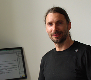
Volcanoes are rarely included in simulations of future climate, because eruptions cannot be predicted. Ingo Bethke used records of past volcanic eruptions from ice cores to insert a range of plausible volcanic events into future climate model projections.
Read more here.

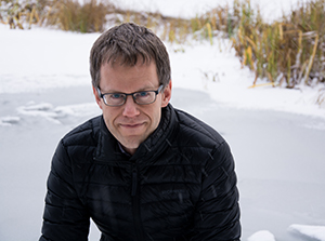
Imagine being at sea in the high north winter time, and suddenly be captured by strong winds, icing and heavy snowfall. There are tales of storms appearing out of nowhere, of a whole fleet of fishermen never coming home. Polar lows are still hard to forecast.
Oskar Landgren models polar lows and their appearance in future climates.
Read more here.
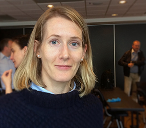
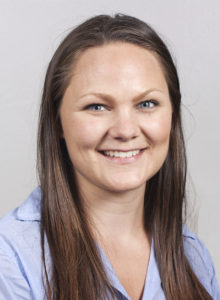
– How sensitive are wetland methane emissions to changes in temperature and precipitation? This is an important question we need answer to get the model right, says Rona L. Thompson.
Thompson is working on inverse modelling for methane emissions in the high latitudes over the past decade.
Read more here.
 Over the sea ice in the Arctic and Antarctica, snow drifts off the ice and into the ocean. Does drifting snow lead to more or less sea ice?
Jens Boldingh Debernard experiments by turning snow drift on and off in the ice module of the Earth system model.
Read more here.
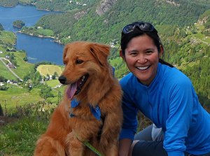
Would you think that looking at a single leaf would have an effect on how you look at global climate?
Hanna Lee looks at individual leaves and sees the important role they play in their surroundings and the way in which we decide to use our land.
Read more here.
Inger Helene Karset uses climate models to study the effect of aerosols and clouds. An eruption from a volcano in 2014 allowed her to compare the clouds in the models with clouds in the real world.
Read more here.